Analyzing free-form text responses in surveys: a 6-step guide
 The biggest topics in a set of free-form text responses to an open question in a survey. The topics emerged from the analysis.
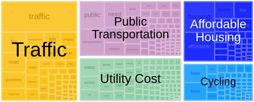
How to analyze free-form text responses
Free-form text responses in surveys are a gold mine of information. Unlike close-ended survey questions, they can be used to spot unexpected narratives and issues that would otherwise have been missed. Instead of asking respondents to choose between a number of preconceived options, open questions allow them to tell their own stories – and for larger narratives to emerge from these individual stories.
When analyzing a Net Promoter Score survey, for example, text analysis can uncover both how people feel about a brand and why they feel that way.
But free-form text responses in surveys are notoriously difficult to analyze. The traditional approach uses text coding, where researchers manually read through and code the responses. This approach suffers from obvious drawbacks, such as being extremely time-consuming and leading to a high risk of ending up with inconsistent codes. Having responses in multiple languages requires researchers with expertise in each language.
An alternative approach involves simple text analysis, like generating a word cloud with the words in the responses. While this can be useful for quickly getting an overview of dominant expressions, it provides little nuance and does not provide any structured output that can be connected to other variables in the data.
This is where Natural Language Understanding comes in. AI-powered topic detection techniques can be used to identify semantically coherent topics in the responses. Sentiment analysis and tonality detection are useful for quantifying the emotional tones expressed. And entity recognition can identify products, brands, and other entities mentioned in the responses.
A step-by-step guide
This post describes a step-by-step process for identifying topics and sentiment in free-form text responses using Dcipher Analytics. We use a public dataset, Community Survey Open-ended Comments (2016 & 2017) conducted by the City of Austin (available as a practice dataset in Dcipher Analytics trial accounts). Respondents have answered the question “If there was ONE thing you could share with the Mayor regarding the City of Austin (any comment, suggestion, etc.), what would it be?”
The whole process took us about 15 minutes. The output includes:
- A table with topics in the responses along with their volume, sentiment, and representative texts
- A foam chart displaying the topics visually
If you just want the fastest way of generating the results, see this tutorial in our Help Center. For more information about each step, keep reading.
Step 1: Import the data
The dataset is in a csv file. We start a blank Dcipher project, upload the data to the Dcipher cloud and import it into the project. Dcipher can handle various file formats, including Excel files, comma- and tab-separated files, and json files.
When importing the dataset into Dcipher, its schema is displayed in the Schema workbench (particularly useful when working with nested data, as tends to quickly become the case when working with text) and the observations are displayed in the Table View.
Step 2: Inspecting the data
Aggregating data gives us a better understanding of the content and helps us spot issues. For example, by dragging the "Year" field to the "Group by" dropzone in the Table View, we get the total number of responses for each year. We see that there are 1,553 responses from 2016 and 1,539 responses from 2017. But we also notice a number of text strings, each with count 1. This is an indication that these rows are misaligned. We therefore apply a filter on the Year field to remove these malformed rows.
A second way of inspecting the data is by looking at individual responses, which can give us insights about possible issues with the data. We do this by opening the Text workbench and dragging the "Comment" field there. In this case, everything looks fine with the data.
Step 3: Splitting the responses into words and phrases
In natural language processing, tokenization is used for dividing text into smaller chunks, called tokens, in a smarter way that through splitting by whitespace. Dcipher's Tokenize & Tag operation offers cleaning of punctuations, emojis, stop words, and short tokens, as well as lowercasing and lemmatization (converting inflection forms of a word into its base form). It also includes options for detecting word phrases, parts-of-speech, and named entities.
Once the tokenization operation has been run, the dataset has now become nested. The original dataset could neatly be displayed in tabular form – each row had a year, a council district, and a comment. But tokenization has created a new field with a collection of tokens, where each token has an id, a value (the word or phrase) and a tag (with the part-of-speech or other tag). This is why at the end of the video above, the "tokens" column shows "[30 items]", "[6 items]", and so on, indicating the number of words or phrases associated with each response.
Let's have a look at a few different ways of making sense of the tokens in Dcipher:
- As a table, showing the id, value, and tag of each token. If we were working with flat structures (think SQL tables), this is what it would look like, with references from the tokens back to the original table with responses.
- As an aggregated list showing each unique token and its number of occurrences in the responses.
- As a token network, where each token is connected to other tokens that it is frequently used in the same comment as. This is similar to a word cloud, but with additional contextual information.
Now that we have split the comments into words and phrases, let's use them to better understand differences in the data. One question we may have is what the key differences are between the comments people gave in 2016 and those from 2017. A quick way of answering that is to look at the words and phrases that are overrepresented in 2016 and 2017 respectively compared to the entire dataset. In other words: what are the words that are used more frequently in 2016 than 2017 and vice versa?
We can see that in 2016, the focus was on traffic solutions ("bring Uber", "light rail") and water problems. In 2017, on the other hand, issues at the top of people's minds included homelessness, CodeNEXT (an initiative to revise regulation on land use in the city), property taxes, and Austin's status as a sanctuary city.
Step 4: Topic modeling
While knowing what words and phrases are used in the free-form text responses can give some information about their content, the vagueness and ambiguity of language means we need further contextual information to actually understand what people are saying. Natural Language Processing offers just the right tool for that: topic modeling.
Topic modeling has been around for a long time, traditionally using statistical approaches such as Latent Dirichlet Allocation (LDA). Dcipher Analytics' toolbox includes such methods, but goes beyond them by also enabling semantic topic modeling. Semantic topic modeling uses word embeddings techniques, where an AI is trained to understand similarity between texts independently of whether they use the same words.
In Dcipher, this is done using the Detect topics operation with the Fast semantic clustering method. If the dataset contains sufficient volumes of text (typically at least 1000 texts), a model can be trained from scratch using the input texts. With a smaller number of posts, a pre-trained model can be used.
In this case we use the default settings, but the settings can be adjusted to search for broader topics/themes.
After identifying topcis in the data, we use the Foam Chart workbench to display the topics and set the filters to limit the number of topics shown.
We can see prominent clusters related to water and electricity fees, public transportation, traffic, the homeless population, expensive rent, high property taxes, and bike lanes, among others.
To get all the relevant information about the topics organized in a single place, we again turn to the Table View to aggregate the data. By grouping by topics and applying aggregation functions, we quickly generate a table showing key information for each topic:
- Number of responses mentioning the topic
- Respondents from which city districts are most prone to mention the topic
- Representative comments related to each topic
Reading the representative comments helps us get a better understanding of each topic.
Step 5: Sentiment analysis
Apart from understanding what people are responding, we also want to understand how they feel about the issues. Dcipher Analytics offers two ways of doing this. One is sentiment analysis, which measures the sentiment of comments on a scale from -1 (strongly negative) to +1 (strongly positive). The other is emojization, which interprets the emotional tone expressed in the text.
For the current analysis we'll use sentiment analysis through Dcipher's Analyze sentiment operation. We then calculate the average sentiment score for each topic and sort the topics by sentiment, starting from the most negative score.
We can see that the traffic situation is the issue that evokes the strongest negative emotions.
Step 6: Exporting the data
Charts as well as data are easy do download in Dcipher. In this case, we want to download the full dataset for further analysis, the table with information about the topics, and the topic foam chart.
Get started!
To access our text analytics toolbox and try out analyzing free-form text responses in Dcipher Analytics, sign up for a free trial.